Centralized, Decentralized and Distributed Control Architecture for Distribution Grid

__author__ = "Andy Putratama"
__website__ = "andyptr.github.io"

Table of contents

1. Introduction
   1. Centralized
   2. Distributed
   3. Decentralized
2. Comparison
   1. Accuracy
   2. Computational Speed
3. Key Takeaways

import pandas as pd
import numpy as np
import matplotlib.pyplot as plt
import algo # Developed package for this project 

1) Introduction

The proposed controller introduced in previous work is a centralized controller, meaning there is a centralized entity (normally a distribution grid operator/DSO ) who is responsible for control and monitoring of the distribution grid.

We can call this entity as a centralized coordinator/controller (CC). We call this a centralized architecture because the CC gathers information from all devices and computes the control action based on the obtained information, all in centralized manner.

In this study, I proposed two addional architectures, namely decentralized and distributed architecture. Furthermore, this study uses the same test case as the previous work, and our aim is to observe the performance of three different architectures by using the exact similar test case and controller parameters.

The illustration of the three different architectures is shown in the following figure.

1. A) Centralized Architecture

For the full description of the centralized architecture (test case, formulation, etc.), please refer to the previous work.

Advantages

Why centralized architecture?

1. Centralized controller is easier to configure and develop. The CC has direct access of information from all devices/houses in the grid, thus controlling the grid will be much simpler, because all information are available.

2. The centralized algorithm is the simplest, compared to the other architectures.

Drawbacks

However, the centralized architecture has major disadvantages:

1. If controller/communication fails, the grid cannot be controlled anymore. The centralized architecture is often called as single-point of failure (SPoF).
2. Privacy issues: This is one of the growing issues nowadays. The CC has direct access and control to all devices (or houses) in the grid. Which indeed will disturb households' privacy.
3. Computationally heavy: Centralized architecture might be preferable for small number of devices. However, with the advancement of technologies, number of devices will increase rapidly in the future. Meaning that one controller has to handle massive amount of devices which may increase the computational cost of the system.
4. Not scalable: Related to point 2. It is not scalable because any installation of new devices will require controller maintenance, which will completely shut off the controller.

Therefore, decentralized and distributed control architectures are developed in order to overcome the challenges faced by centralized architecture.

Run Centralized Controller

As explained previously, we aim to compare the centralized architecture with distributed and decentralized architectures. Therefore, let's firstly run the OPF with centralized architecture.

I use the following grid and parameter data for the three controllers

data_dir = "data/33bus_PV.xlsx"
param = {"S_base": 20, # Base MVA
         "V_base" : 12.66, # Base voltage (based on IEEE 33 bus)
         "V_min" : 0.95, # Min operating voltage
         "V_max" : 1.05, # Max operating voltage
         "c_pv" : .5, # Cpv in the objective function
        "c_loss" : 1} # Closs in the objective function

Firstly, run the centralized controller

bus, branch = algo.load_data.opf_data(data_dir, param)

bus_centralized, branch_centralized, time_centralized = algo.solve.centralized(bus.copy(), branch.copy(), param)

The results will be compared in the next section.

1. B) Distributed Architecture

In distributed architecture, there is no centralized coordinator. But, all the devices/houses are the controller themselves. In this case, the devices/houses are also called as control agents. Figure below illustrates the distributed architecture. Note that the green dashed-lines refer to the communication flows.

In this architecture, each house only knows its local information and doesn't know anything about the global state of the grid.

In order to control globally the grid, all houses then actively communicate with each other. However, the communication is limited, in which each house can only communicate with its neighbors.

The control and the communication schemes follow a distributed alogrithm called alternating direction method of multipliers (ADMM). The formulation of this architecture is explained in my publication [1]

^{Ref: [1] M. A. Putratama, R. Rigo-Mariani, V. Debusschere and Y. Besanger, "Parameter Tuning for LV Centralized and Distributed Voltage Control with High PV Production," 2021 IEEE Madrid PowerTech, 2021, pp. 1-6, doi: 10.1109/PowerTech46648.2021.9494802.}

Advantages

The distributed architecture overcomes the challenges of centralized architecture.

1. No single point of failure: If any control agents (houses) fails, other houses can still operate.
2. Limit privacy concerns: There is no centralized entity anymore, and houses only communicate limited amount of information/variables to their neighbors
3. scalable.
4. computational sharing: with distributed control, the computation can be shared to the houses.

Drawbacks

1. More complicated algorithm.
2. All devices/houses are required to have computational capability. In other words, more investments are needed.
3. Long computational time: Longer time to reach the optimality (convergence), which will be explained in the next section.

Run Distributed Controller

I use the same test case as the previous work (IEEE 33 bus). In this architecture, all 33 buses are the control agents.

bus_distributed, branch_distributed, time_distributed, residuals_distributed = algo.solve.distributed(bus.copy(), branch.copy(), param)

1. C) Decentralized Architecture

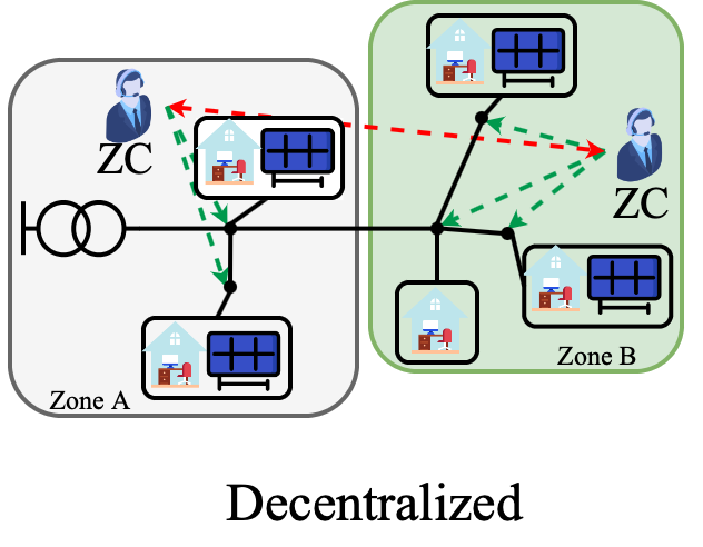
In decentralized architecture, the grid is divided into several zones and each zone is monitored and controller by a zone coordinator (ZC) (thus ZC = control agent), as illustrated below:

The ZC only has access to devices/information within its zone, and ZC control its zone in the similar way as CC in the centralized architecture.

Similar to distributed architecture, all the ZCs are actively communicating with their neighboring ZCs to control the grid globally. The control and the communication schemes also follow ADMM principles.

Unfortunately, detailed formulation of the decentralized algorithm is not presented in this noteboook, because it is still an ungoing publication.

Advantages & Drawbacks

Decentralized control is the intermediary state between centralized and distributed control.

It still has SPoF characteristic for zones, but it can improve the limitations of centralized control (nevertheless, distributed control is still better!)

One of the main consideration of using decentralized control to distributed control is the computational speed, which is significantly faster. We will see this comparison in the next section.

Run Decentralized Controller

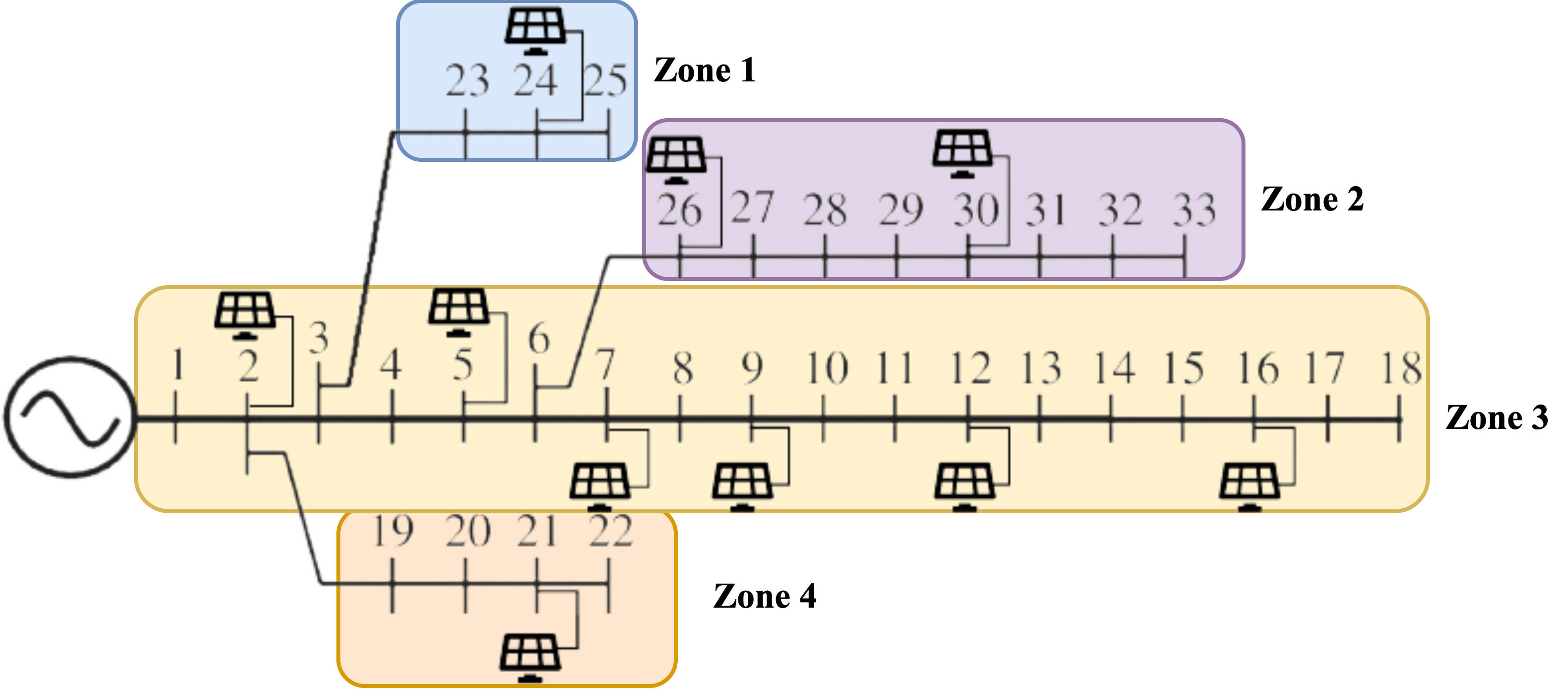
For decentralized control, the IEEE 33 bus is partitioned to 4 zones, as follow.

bus_decentralized, branch_decentralized, time_decentralized, residuals_decentralized = algo.solve.decentralized(bus.copy(), branch.copy(), param)

2) Performance Comparisons

2. A) Accuracy

# Create figure and axis
fig, (ax) = plt.subplots(nrows=1, ncols=1, figsize= (3.2, 1), dpi = 700)
csfont = {'fontname': 'Times New Roman'}


# Centralized
ax.plot(bus_centralized['voltage'], linestyle = '--',  linewidth = 0.5,marker = "1", markersize = 5, 
        alpha=1, mec='green', mfc = "green", color ="deepskyblue",  label = "Centralized")
# Distributed
ax.plot(bus_distributed['voltage'], linestyle = '--',  linewidth = 0.5, marker = "2", markersize = 5, 
        alpha=1, mec='orange', mfc = "orange", color ="sandybrown",  label = "Decentralized")
# Decentralized
ax.plot(bus_decentralized['voltage'], linestyle = '--',  linewidth = 0.5,marker = "3", markersize = 5, 
        alpha=1, mec='royalblue', mfc = "royalblue", color ="tomato", label = "Distributed")

ax.plot(bus_centralized.index, [1.05 for _ in bus_centralized.index],
        linestyle = "-.",linewidth = .5, alpha=1, color ="k", label = "Voltage limit")



ax.autoscale(enable=True, axis='y', tight=True)



# modify font 
for tick in ax.get_yticklabels():
    tick.set_fontname("Times New Roman")
    tick.set_fontsize(7)

for tick in ax.get_xticklabels():
    tick.set_fontname("Times New Roman")
    tick.set_fontsize(7)
    tick.set_rotation(0)
    
ax.set_ylabel('Voltage (p.u.)', fontsize=6, **csfont,)
ax.set_xlabel('Bus', fontsize=6, **csfont)
ax.set_title('Voltage Profile Comparison', fontsize=7, **csfont)


ax.autoscale(enable=True, axis='x', tight=True)
ax.set_xticks(np.arange(0, 33, 4))
ax.set_xticklabels(np.arange(0, 33, 4)+1)
ax.set_yticks([1, 1.025, 1.05, 1.075, 1.1])

ax.grid(axis= "y", color = 'k', linestyle = '-.', alpha = 0.5, linewidth = 0.1)
ax.grid(axis= "x", color = 'k', linestyle = '-.', alpha = 0.5, linewidth = 0.1)
ax.autoscale(enable=True, axis='x', tight=True)

leg = ax.legend(fancybox=True, framealpha=0.5, loc='lower center', bbox_to_anchor=(0.7, 0.6), 
                ncol = 2, prop={'family': 'Times New Roman', 'size': 5},
               handletextpad=0.3, handlelength=1, columnspacing=0.7,)

Based on the above voltage profile, we can see all controllers obtained the exactly the same voltage profile.

Now lets try to compare the PV curtailments:

fig, (ax) = plt.subplots(nrows=1, ncols=1, figsize= (3.2, 1), dpi = 700)
csfont = {'fontname': 'Times New Roman'}

bar_width = 0.2
bus_with_pv = bus[bus["S_PV"] > 0].index

ax.bar(np.array([pv for pv in range(len(bus_centralized.index[bus_with_pv]))]), 
       bus_centralized["curt"].values[bus_with_pv], width = bar_width, 
       color = "deepskyblue", label = 'Centralized')

ax.bar(np.array([pv for pv in range(len(bus_distributed.index[bus_with_pv]))]) + bar_width, 
       bus_distributed["curt"].values[bus_with_pv], width = bar_width, 
       color = "sandybrown", label = "Distributed")   

ax.bar(np.array([pv for pv in range(len(bus_decentralized.index[bus_with_pv]))]) + bar_width*2, 
       bus_decentralized["curt"].values[bus_with_pv], width = bar_width, 
       color = "tomato", label = "Decentralized") 

ax.set_xticks(np.array([pv for pv in range(len(bus_centralized.index[bus_with_pv]))]) + .2)
ax.set_xticklabels(bus_with_pv + 1)

ax.set_yticks(np.arange(0,101, 25))

ax.grid(axis= "y", color = 'k', linestyle = '-.', alpha = 0.5, linewidth = 0.1)
ax.grid(axis= "x", color = 'k', linestyle = '-.', alpha = 0.5, linewidth = 0.1)

# modify font 
for tick in ax.get_yticklabels():
    tick.set_fontname("Times New Roman")
    tick.set_fontsize(7)

for tick in ax.get_xticklabels():
    tick.set_fontname("Times New Roman")
    tick.set_fontsize(7)
    tick.set_rotation(0)
    
ax.set_ylabel('PV Curtailments (%)', fontsize=6, **csfont,)
ax.set_xlabel('Bus with PV', fontsize=6, **csfont)
ax.set_title('Active Power Curtailment Comparison', fontsize=7, **csfont)

ax.autoscale(enable=True, axis='x', tight=True)

leg = ax.legend(fancybox=True, framealpha=0.5, loc='lower center', bbox_to_anchor=(0.8, 0.5), 
                ncol = 1, prop={'family': 'Times New Roman', 'size': 5},
               handletextpad=0.3, handlelength=1, columnspacing=0.7,)

As we can see, the controllers obtained the similar PV curtailments as well. This simulation highlights that the proposed distributed algorithm implemented in both distributed and decentralized architecture can completely transform a centralized problem into distributed or decentralized problem, without affecting any computational behavior/results of the controller.

2. B) Computational Speed

As the distributed and decentralized control are iterative algorithm, their computational speed refers to the time needed to reach convergence criteria. The computational speed of the three controllers are:

f"centralized: {time_centralized} s, distributed: {time_distributed} s, decentralized: {time_decentralized} s"

'centralized: 0.49 s, distributed: 700.82 s, decentralized: 47.54 s'

As we can see, the main advantage of the centralized control is the computational time. The distributed control took 15x longer than the decentralized control.

We can see clearly the tradeoff here that the more distributed the architecture, the more computational time is required.

The longer computational time is due to the iterative nature of the distributed algorithm. As opossed to centralized architecture, the distributed (and decentralized) algorithm uses iterative process to solve the OPF. Hence, the more control agent (distributed = 33 agents, while decentralized = 4 agents/zones), the more time it requires for the controller to solve the OPF.

The iterative process can be observed by looking at the residuals of both controllers.

# Create figure and axis
fig, (ax, ax2) = plt.subplots(nrows=2, ncols=1, figsize= (3.2, 2), dpi = 700, sharex=True,)
csfont = {'fontname': 'Times New Roman'}

################################### Distributed ########################################


# Primal Residual
ax.plot(residuals_distributed.loc[(slice(None), "primal"), :].sum(), linestyle = '-',  
        color ="deepskyblue",  label = "Primal")
# Dual Residual
ax.plot(residuals_distributed.loc[(slice(None), "dual"), :].sum(), linestyle = '--',  linewidth = 0.5, 
        color ="sandybrown",  label = "Dual")

ax.autoscale(enable=True, axis='y', tight=True)

# modify font 
for tick in ax.get_yticklabels():
    tick.set_fontname("Times New Roman")
    tick.set_fontsize(7)

for tick in ax.get_xticklabels():
    tick.set_fontname("Times New Roman")
    tick.set_fontsize(7)
    tick.set_rotation(0)
    
ax.set_ylabel('Residuals', fontsize=6, **csfont,)
ax.set_title('Distributed Control Residuals', fontsize=7, **csfont)


ax.autoscale(enable=True, axis='x', tight=True)
ax.annotate('Convergence criteria reached',
            xy=(800, 0), xycoords='data',
            xytext=(-25, 20), textcoords='offset points',size = 5,
            arrowprops=dict(arrowstyle="->", lw = .5,), **csfont)

ax.grid(axis= "y", color = 'k', linestyle = '-.', alpha = 0.5, linewidth = 0.1)
ax.grid(axis= "x", color = 'k', linestyle = '-.', alpha = 0.5, linewidth = 0.1)
ax.autoscale(enable=True, axis='x', tight=True)

leg = ax.legend(fancybox=True, framealpha=0.5, loc='lower center', bbox_to_anchor=(0.7, 0.6), 
                ncol = 2, prop={'family': 'Times New Roman', 'size': 5},
               handletextpad=0.3, handlelength=1, columnspacing=0.7,)
fig.subplots_adjust(hspace=0.8)


################################### Decentralized ########################################

# Primal Residual
ax2.plot(residuals_decentralized.loc[(slice(None), "primal"), :].sum(), linestyle = '-',  
        color ="deepskyblue",  label = "Primal")
# Dual Residual
ax2.plot(residuals_decentralized.loc[(slice(None), "dual"), :].sum(), linestyle = '--',  linewidth = 0.5, 
        color ="sandybrown",  label = "Dual")

ax2.autoscale(enable=True, axis='y', tight=True)

# modify font 
for tick in ax2.get_yticklabels():
    tick.set_fontname("Times New Roman")
    tick.set_fontsize(7)

for tick in ax2.get_xticklabels():
    tick.set_fontname("Times New Roman")
    tick.set_fontsize(7)
    tick.set_rotation(0)
    
ax2.set_ylabel('Residuals', fontsize=6, **csfont,)
ax2.set_xlabel('Iteration Number', fontsize=6, **csfont)
ax2.set_title('Decentralized Control Residuals', fontsize=7, **csfont)


ax2.autoscale(enable=True, axis='x', tight=True)
ax2.annotate('Convergence criteria reached',
            xy=(60, 0), xycoords='data',
            xytext=(20, 20), textcoords='offset points',size = 5,
            arrowprops=dict(arrowstyle="->", lw = .5,), **csfont)

ax2.grid(axis= "y", color = 'k', linestyle = '-.', alpha = 0.5, linewidth = 0.1)
ax2.grid(axis= "x", color = 'k', linestyle = '-.', alpha = 0.5, linewidth = 0.1)
ax2.autoscale(enable=True, axis='x', tight=True)

leg = ax2.legend(fancybox=True, framealpha=0.5, loc='lower center', bbox_to_anchor=(0.7, 0.6), 
                ncol = 2, prop={'family': 'Times New Roman', 'size': 5},
               handletextpad=0.3, handlelength=1, columnspacing=0.7,)

The convergence criteria is the criteria where the iteration can be stopped i.e., when the iteration reach the convergence.

As we can see in the figure above, the decentralized control reached the convergence criteria around 50 iterations, while distributed control in 800 iterations. Which then highlight the more control agents, the more iterations required for the algorithm to reach the connvergence criteria.

3) Key Takeaways

We have seen that the proposed distributed algorithm can effectively transform the centralized problem into distributed or decentralized problem.

We've seen also the drawback of moving towards the distributed control is the computational time. Furthermore, there are still more limitations to move to distributed control that are not considered in this study. For instance:

1. Investments in infrastructure (communication, devices) should be considered.
2. Communication limitation (communication bandwith)
3. Willingness of the houseowners to participate in distributed control. This might be linked to privacy concerns.

So, which architecture is the best?

It depends on the situation. For instance:

1. If distribution grid consists of small nodes/devices ==> centralized architecture might be better
2. If there are lot of nodes ==> Distributed/decentralized
   • However, we have to be careful on the computational time!
3. To limit information sharing (preserve prosumers privacy) ==> Distributed control