Improving Grid Impedance Estimation Using Model Fitting

__author__ = "Andy Putratama"
__website__ = "andyptr.github.io"

Table of contents

1. Introduction
2. Using Estimated Data for Operational Planning
3. Proposed Model Fitting Algorithm
4. Key Takeaways

import pandas as pd
import numpy as np
import matplotlib.pyplot as plt
import algo # Developed package for this project 

1) Introduction

The voltage control I have developed in previous studies are model based controllers, which rely fully on grid data (i.e., line impedance data).

However in real-life, distribution grid data is usually not available/hard to obtain, especially for low-voltage grid.

In this study, I develop a model fitting algorithm to compute line impedance using historic measurement data.

The test case used in this study is a 11-bus distribution grid, as shown in figure below:

In the test case, we use a centralized controller to control the battery (the PV is not controllable/cannot be curtailed) in order to maintain the grid voltage.

We consider one-day simulation/operation with 30 minutes time step. The controller then aims to optimize the battery for the full one day of operation.

In the first step of the simulation, we do not have any knowledge of the line impedance. Thus, I use a rough estimation for the impedance value. This point will be explained further in the next section.

Firstly, let's load the grid data and PV profile:

real_grid_dir = "data/7bus/grid_data.xlsx" # Grid data
load_profile_dir = "data/7bus/load_profile_1day.csv" # load profile
pv_profile_dir = "data/7bus/PV_profile_1day.csv" # PV profile

Load the data & profile

bus_data, branch_data, load_profile, pv_profile = algo.load_data.grid_data(real_grid_dir, load_profile_dir, pv_profile_dir)

Let's look on the PV profile:

# Create figure and axis
fig, (ax) = plt.subplots(nrows=1, ncols=1, figsize= (3.2, 1), dpi = 700)
csfont = {'fontname': 'Times New Roman'}


# Plot PV Profile
for bus in pv_profile.columns:
    ax.plot(pv_profile[bus], linestyle = '-',  linewidth = 1, label = f"Bus {bus}")

ax.autoscale(enable=True, axis='y', tight=True)


# modify font 
for tick in ax.get_yticklabels():
    tick.set_fontname("Times New Roman")
    tick.set_fontsize(7)

for tick in ax.get_xticklabels():
    tick.set_fontname("Times New Roman")
    tick.set_fontsize(7)
    tick.set_rotation(0)
    
ax.set_ylabel('PV Active Power (MW)', fontsize=6, **csfont,)
ax.set_xlabel('Bus', fontsize=6, **csfont)
ax.set_title('PV Profile', fontsize=7, **csfont)


ax.autoscale(enable=True, axis='x', tight=True)

# Set x ticks
ax.set_xticks([pv_profile.index[t] for t in range(len(pv_profile.index)) if t%8 == 0])
ax.set_xticklabels([str(pv_profile.index[t].time()) for t in range(len(pv_profile.index)) if t%8 == 0])

# set y ticks
ax.set_yticks([0, 0.05, 0.1, 0.15, 0.2])

ax.grid(axis= "y", color = 'k', linestyle = '-.', alpha = 0.5, linewidth = 0.1)
ax.grid(axis= "x", color = 'k', linestyle = '-.', alpha = 0.5, linewidth = 0.1)
ax.autoscale(enable=True, axis='x', tight=True)

leg = ax.legend(fancybox=True, framealpha=0.5, loc='lower center', bbox_to_anchor=(0.8, 0.4), 
                ncol = 1, prop={'family': 'Times New Roman', 'size': 5},
               handletextpad=0.3, handlelength=1, columnspacing=0.7,)

And the load profile:

# Create figure and axis
fig, (ax) = plt.subplots(nrows=1, ncols=1, figsize= (3.2, 1), dpi = 700)
csfont = {'fontname': 'Times New Roman'}


# Plot PV Profile
for bus in load_profile.columns:
    ax.plot(load_profile[bus], linestyle = '-',  linewidth = 1, label = f"Bus {bus}")

ax.autoscale(enable=True, axis='y', tight=True)


# modify font 
for tick in ax.get_yticklabels():
    tick.set_fontname("Times New Roman")
    tick.set_fontsize(7)

for tick in ax.get_xticklabels():
    tick.set_fontname("Times New Roman")
    tick.set_fontsize(7)
    tick.set_rotation(0)
    
ax.set_ylabel('Load Active Power (MW)', fontsize=6, **csfont,)
ax.set_xlabel('Bus', fontsize=6, **csfont)
ax.set_title('Load Profile', fontsize=7, **csfont)


ax.autoscale(enable=True, axis='x', tight=True)

# Set x ticks
ax.set_xticks([pv_profile.index[t] for t in range(len(pv_profile.index)) if t%8 == 0])
ax.set_xticklabels([str(pv_profile.index[t].time()) for t in range(len(pv_profile.index)) if t%8 == 0])

# set y ticks
ax.set_yticks([0, 0.05, 0.1, 0.15, 0.2])

ax.grid(axis= "y", color = 'k', linestyle = '-.', alpha = 0.5, linewidth = 0.1)
ax.grid(axis= "x", color = 'k', linestyle = '-.', alpha = 0.5, linewidth = 0.1)
ax.autoscale(enable=True, axis='x', tight=True)

leg = ax.legend(fancybox=True, framealpha=0.5, loc='lower center', bbox_to_anchor=(0.5, 0.8), 
                ncol = 6, prop={'family': 'Times New Roman', 'size': 5},
               handletextpad=0.3, handlelength=1, columnspacing=0.7,)

2) Operational Planning with Estimated Data

To recall, our main objective is to maintain the grid voltage over the day using batteries. To do so, I developed a voltage control / optimization algorithm that takes into account battery operation. The proposed voltage control was adapted based on my previous work. The full formulation of the controller is not yet available because it is still an ongoing publication.

In the first step of this study, we try to use estimated grid (line impedance) data to optimize the grid operation, because the real/actual data is not available.

Let's open our estimated data:

grid_data_estimate_dir = "data/7bus/data_estimate.xlsx"
bus_data_estimated , branch_data_estimated = algo.load_data.grid_data_estimate(grid_data_estimate_dir)

Now, let's see the difference between the estimated data that we will use for optimization and the actual data:

fig, (ax, ax2) = plt.subplots(nrows=2, ncols=1, figsize= (3.2, 2), dpi = 700, sharex=True)
csfont = {'fontname': 'Times New Roman'}

x_axis = np.arange(len(branch_data.index))+1
bar_width = 0.4

########################## 1st Subplot #################################
# Real data
ax.bar(x_axis, 
       branch_data["r"].values, width = bar_width, 
       color = "forestgreen", label = 'Actual')

# Estimated data
ax.bar(x_axis + bar_width, 
       branch_data_estimated["r"].values, width = bar_width, 
       color = "sandybrown", label = "Estimated")   

# add 2nd Y axis
ax1 = ax.twinx()

# calculate absolute error
y_error = 100*np.abs((branch_data["r"].values - branch_data_estimated["r"].values)/branch_data["r"].values)
ax1.plot(x_axis, y_error,  linestyle = '-.', linewidth = 0.5, marker = ".", markersize = 2, 
        alpha=1, mec='red', mfc = "red", color ="k", label = "absolute error")


# set x axis ticks
ax.set_xticks(x_axis + .2)
ax.set_xticklabels(x_axis)

# set y axis ticks
ax.set_yticks([0, 0.3, 0.6, 0.9])
ax1.set_yticks([0, 25, 50, 75])


ax.grid(axis= "y", color = 'k', linestyle = '-.', alpha = 0.5, linewidth = 0.1)
ax.grid(axis= "x", color = 'k', linestyle = '-.', alpha = 0.5, linewidth = 0.1)

# modify font 
for tick in ax.get_yticklabels():
    tick.set_fontname("Times New Roman")
    tick.set_fontsize(7)

for tick in ax.get_xticklabels():
    tick.set_fontname("Times New Roman")
    tick.set_fontsize(7)
    tick.set_rotation(0)
    
for tick in ax1.get_yticklabels():
    tick.set_fontname("Times New Roman")
    tick.set_fontsize(7)


    
ax.set_ylabel('Resistance (Ohm)', fontsize=6, **csfont,)
ax.set_title('Comparison Between Actual vs Estimated Line Resistance', fontsize=7, **csfont)
ax1.set_ylabel('Absolute Error (%)', fontsize=6, **csfont,)



ax1.autoscale(enable=True, axis='x', tight=True)

leg = ax.legend(fancybox=True, framealpha=0.5, loc='lower center', bbox_to_anchor=(0.85, 0.5), 
                ncol = 1, prop={'family': 'Times New Roman', 'size': 5},
               handletextpad=0.3, handlelength=1, columnspacing=0.7,)
ax1.legend(fancybox=True, framealpha=0.5, loc='lower center', bbox_to_anchor=(0.85, 0.2), 
                ncol = 1, prop={'family': 'Times New Roman', 'size': 5},
               handletextpad=0.3, handlelength=1, columnspacing=0.7,)

fig.subplots_adjust(hspace=0.8)


########################## 2nd Subplot #################################
# Real data
ax2.bar(x_axis, 
       branch_data["x"].values, width = bar_width, 
       color = "forestgreen", label = 'Actual')

# Estimated data
ax2.bar(x_axis + bar_width, 
       branch_data_estimated["x"].values, width = bar_width, 
       color = "sandybrown", label = "Estimated")   

# add 2nd Y axis
ax3 = ax2.twinx()

# calculate absolute error
y_error = 100*np.abs((branch_data["x"].values - branch_data_estimated["x"].values)/branch_data["x"].values)
ax3.plot(x_axis, y_error,  linestyle = '-.', linewidth = 0.5, marker = ".", markersize = 2, 
        alpha=1, mec='red', mfc = "red", color ="k", label = "absolute error")


# set x axis ticks
ax2.set_xticks(x_axis + .2)
ax2.set_xticklabels(x_axis)

# set y axis ticks
ax2.set_yticks([0, 0.2, 0.4, 0.6])
ax3.set_yticks([0, 30, 60, 90])


ax2.grid(axis= "y", color = 'k', linestyle = '-.', alpha = 0.5, linewidth = 0.1)
ax2.grid(axis= "x", color = 'k', linestyle = '-.', alpha = 0.5, linewidth = 0.1)

# modify font 
for tick in ax2.get_yticklabels():
    tick.set_fontname("Times New Roman")
    tick.set_fontsize(7)

for tick in ax2.get_xticklabels():
    tick.set_fontname("Times New Roman")
    tick.set_fontsize(7)
    tick.set_rotation(0)
    
for tick in ax3.get_yticklabels():
    tick.set_fontname("Times New Roman")
    tick.set_fontsize(7)


    
ax2.set_ylabel('Reactance (Ohm)', fontsize=6, **csfont,)
ax2.set_xlabel('Line Index', fontsize=6, **csfont)
ax2.set_title('Comparison Between Actual vs Estimated Line Reactance', fontsize=7, **csfont)
ax3.set_ylabel('Absolute Error (%)', fontsize=6, **csfont,)



ax2.autoscale(enable=True, axis='x', tight=True)

leg = ax2.legend(fancybox=True, framealpha=0.5, loc='lower center', bbox_to_anchor=(0.2, 0.6), 
                ncol = 2, prop={'family': 'Times New Roman', 'size': 5},
               handletextpad=0.3, handlelength=1, columnspacing=0.7,)
ax3.legend(fancybox=True, framealpha=0.5, loc='lower center', bbox_to_anchor=(0.85, 0.6), 
                ncol = 1, prop={'family': 'Times New Roman', 'size': 5},
               handletextpad=0.3, handlelength=1, columnspacing=0.7,)

<matplotlib.legend.Legend at 0x7f8028d916a0>

Figure above shows the difference between the actual data of line resistance (top) and the reactance (bottom) and the dashed lines represent the absolute error between the actual and the estimated data.

Note that line 3 has very small resistance and reactance, thus we cannot see clearly in the bar chart. As we can see, our estimation is not perfect, with some lines can reach absolute error above 50 %.

This situation may happen in real life, since grid data is oftenly not available.

Now, let's see what happen if we use our estimated data to control the grid operation.

We use the following controller parameters:

param = {"V_min" : 0.95, # Min operating voltage
         "V_max" : 1.05, # Max operating voltage,
         "V_low" : 0.9, # Min voltage bound
         "V_high" : 0.9, # max voltage bound
         "Closs"  : 1, # Closs weight function
         "Cvolt" : 0.5} # Cvolt weight function

Note that the parameters used here are different than the two previous studies.

Now run the controller:

voltage_expected_init, SoC_init, battery_setpoints_init = algo.solve.OPF_mpc(bus_data_estimated, branch_data_estimated, param)

The output of the controller is battery operational schedule for one day, which are battery state-of-charge (SoC) and battery power setpoints. Moreover, the controller also internally calculate the expected grid voltage.

The battery SoC:

# Create figure and axis
fig, (ax) = plt.subplots(nrows=1, ncols=1, figsize= (3.2, 1), dpi = 700)
csfont = {'fontname': 'Times New Roman'}

# Plot PV Profile
for bus in SoC_init.columns:
    ax.plot(SoC_init[bus], linestyle = '-',  linewidth = .5, label = f"Bus {bus}")

ax.autoscale(enable=True, axis='y', tight=True)


# modify font 
for tick in ax.get_yticklabels():
    tick.set_fontname("Times New Roman")
    tick.set_fontsize(7)

for tick in ax.get_xticklabels():
    tick.set_fontname("Times New Roman")
    tick.set_fontsize(7)
    tick.set_rotation(0)
    
ax.set_ylabel('SoC (%)', fontsize=6, **csfont,)
ax.set_xlabel('Bus', fontsize=6, **csfont)
ax.set_title('Battery SoC (Estimated data)', fontsize=7, **csfont)


ax.autoscale(enable=True, axis='x', tight=True)

# Set x ticks
ax.set_xticklabels([str(pv_profile.index[t].time()) for t in range(len(pv_profile.index)) if t%8 == 0])

# set y ticks
ax.set_yticks([0, 20, 40, 60, 80, 100])

ax.grid(axis= "y", color = 'k', linestyle = '-.', alpha = 0.5, linewidth = 0.1)
ax.grid(axis= "x", color = 'k', linestyle = '-.', alpha = 0.5, linewidth = 0.1)
ax.autoscale(enable=True, axis='x', tight=True)

leg = ax.legend(fancybox=True, framealpha=0.5, loc='lower center', bbox_to_anchor=(0.8, 0.1), 
                ncol = 2, prop={'family': 'Times New Roman', 'size': 5},
               handletextpad=0.3, handlelength=1, columnspacing=0.7,)

<ipython-input-11-b63626060b5b>:30: UserWarning: FixedFormatter should only be used together with FixedLocator
  ax.set_xticklabels([str(pv_profile.index[t].time()) for t in range(len(pv_profile.index)) if t%8 == 0])

Now, let's use the obtained intial battery setpoints in the actual operation (load flow simulation):

measurements_init = algo.solve.load_flow_one_day(bus_data_estimated, branch_data_estimated, 
                                                 load_profile, pv_profile, battery_setpoints_init)

To assess the accuracy of the estimated impedance, we can compare the expected voltage computed by the controller and the actual voltage measurements (from load flow).

For each time step, the voltage error (in %) can be calculated by using the following formula [1]:

^{Ref: [1] R. Rigo-Mariani, V. Debusschere and M. -C. Alvarez-Herault, "A Modified DistFlow for Distributed Generation Planning Problems in Radial Grids," IECON 2020 The 46th Annual Conference of the IEEE Industrial Electronics Society, 2020, pp. 1626-1632, doi: 10.1109/IECON43393.2020.9254865.}

$$\large{\Delta V (\%) = \frac{100}{\text{nb of bus}} \sum_{i \in N} \frac{\vert V_i - V_i^* \vert}{\frac{1}{\text{nb of bus}} \sum_{i \in N} \vert 1 - V_i^* \vert} }$$

Where V^* denotes the measurement voltage.

We can then create a voltage error data frame:

Verror = pd.DataFrame(index = voltage_expected_init.index, columns = ["init", "fitted"])

Create voltage error for estimated data

for idx in Verror.index:
    Verror.loc[idx, "init"] = (100/len(voltage_expected_init.columns))*(np.abs(voltage_expected_init.loc[idx] - measurements_init[0].loc[idx])/(1/(len(measurements_init[0].columns)) * np.abs(1 - measurements_init[0].loc[idx]).sum())).sum()

Plot the error:

fig, (ax) = plt.subplots(nrows=1, ncols=1, figsize= (3.2, 1), dpi = 700, sharex=True)
csfont = {'fontname': 'Times New Roman'}

x_axis = np.arange(len(Verror.index))
bar_width = 0.5

# Verror data
ax.plot(x_axis, Verror["init"].values,  linestyle = '--',  linewidth = 0.5, marker = "*", markersize = 2, 
        alpha=1, mec='orange', mfc = "orange", color ="sandybrown",)

#set x axis ticks
ax.set_xticks([x for x in x_axis if x%8 == 0 ])
ax.set_xticklabels([str(pv_profile.index[t].time()) for t in range(len(pv_profile.index)) if t%8 == 0])


# set y axis ticks
#ax.set_yticks([0, 0.3, 0.6, 0.9])


ax.grid(axis= "y", color = 'k', linestyle = '-.', alpha = 0.5, linewidth = 0.1)
ax.grid(axis= "x", color = 'k', linestyle = '-.', alpha = 0.5, linewidth = 0.1)

# modify font 
for tick in ax.get_yticklabels():
    tick.set_fontname("Times New Roman")
    tick.set_fontsize(7)

for tick in ax.get_xticklabels():
    tick.set_fontname("Times New Roman")
    tick.set_fontsize(7)
    tick.set_rotation(0)
    
for tick in ax1.get_yticklabels():
    tick.set_fontname("Times New Roman")
    tick.set_fontsize(7)


ax.set_xlabel('Time', fontsize=6, **csfont,)
ax.set_ylabel('Absolute Error (%)', fontsize=6, **csfont,)
ax.set_title('Voltage Estimation Error Over The Day', fontsize=7, **csfont)

ax.autoscale(enable=True, axis='x', tight=True)

We can see that the absolute estimated voltage error is around 20% over the time.

To see clearly the error, let's observe voltage profile of one of the nodes:

fig, (ax) = plt.subplots(nrows=1, ncols=1, figsize= (3.2, 1), dpi = 700, sharex=True)
csfont = {'fontname': 'Times New Roman'}

x_axis = np.arange(len(Verror.index))
bar_width = 0.5

# Verror data
ax.plot(x_axis, voltage_expected_init["11"].values,  linestyle = '-',  linewidth = 0.5, color ="sandybrown", label = "controller estimation")
ax.plot(x_axis, measurements_init[0]["11"].values,  linestyle = '-',  linewidth = 0.5, color ="forestgreen", label = "real measurement")
#set x axis ticks
ax.set_xticks([x for x in x_axis if x%8 == 0 ])
ax.set_xticklabels([str(pv_profile.index[t].time()) for t in range(len(pv_profile.index)) if t%8 == 0])


# set y axis ticks

ax.grid(axis= "y", color = 'k', linestyle = '-.', alpha = 0.5, linewidth = 0.1)
ax.grid(axis= "x", color = 'k', linestyle = '-.', alpha = 0.5, linewidth = 0.1)

# modify font 
for tick in ax.get_yticklabels():
    tick.set_fontname("Times New Roman")
    tick.set_fontsize(7)

for tick in ax.get_xticklabels():
    tick.set_fontname("Times New Roman")
    tick.set_fontsize(7)
    tick.set_rotation(0)
    
for tick in ax1.get_yticklabels():
    tick.set_fontname("Times New Roman")
    tick.set_fontsize(7)

ax.autoscale(enable=True, axis='x', tight=True)
ax.set_xlabel('Time', fontsize=6, **csfont,)
ax.set_ylabel('Voltage (p.u.)', fontsize=6, **csfont,)
ax.set_title('Voltage Profile at Bus 11 with Initial Estimated Impedance', fontsize=7, **csfont)


leg = ax.legend(fancybox=True, framealpha=0.5, loc='lower center', bbox_to_anchor=(0.85, 0.5), 
                ncol = 1, prop={'family': 'Times New Roman', 'size': 5},
               handletextpad=0.3, handlelength=1, columnspacing=0.7,)

We can see clearly the gap of error between the controller's estimation and the real measurement.

We can see the controller expected the voltage to always be above the lower limit (0.95 p.u.). However, due to inacuraccy of the estimated impedance, the real voltage at bus 11 happens to be lower than the expected, resulting in undervoltage between 16:00 until midnight.

3) Proposed Model Fitting Algorithm

The aim of model fitting algorithm is to improve the accuracy of the estimated impedance, by using historical measurement data.

The algorithm works as follow:

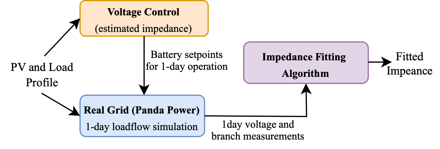
In principal:

1. Firstly, we use the initial estimated grid impedance to optimize the grid for a day (the time horizon could be less/more).
2. Then we use the actual measurement data as the input of the proposed fitting algorithm
3. The fitting algorithm will give the new estimated impedance (we will call it fitted impedance)
4. The fitted impedance then will be used to optimize the next following days.

In the previous simulation, we have obtained the actual measurement data. Let's use that measurement data in the proposed fitting algorithm:

branch_data_fitted = algo.solve.model_fitting(bus_data_estimated, branch_data_estimated, measurements_init)

Now, let's see the comparison between the obtained fitted impedance with the actual impedance:

fig, (ax, ax2) = plt.subplots(nrows=2, ncols=1, figsize= (3.2, 2), dpi = 700, sharex=True)
csfont = {'fontname': 'Times New Roman'}

x_axis = np.arange(len(branch_data.index))+1
bar_width = 0.4

########################## 1st Subplot #################################
# Real data
ax.bar(x_axis, 
       branch_data["r"].values, width = bar_width, 
       color = "forestgreen", label = 'Actual')

# Estimated data
ax.bar(x_axis + bar_width, 
       branch_data_fitted["r"].values, width = bar_width, 
       color = "deepskyblue", label = "Fitted")   

# add 2nd Y axis
ax1 = ax.twinx()

# calculate absolute error
y_error = 100*np.abs((branch_data["r"].values - branch_data_fitted["r"].values)/branch_data["r"].values)
ax1.plot(x_axis, y_error,  linestyle = '-.', linewidth = 0.5, marker = ".", markersize = 2, 
        alpha=1, mec='red', mfc = "red", color ="k", label = "absolute error")


# set x axis ticks
ax.set_xticks(x_axis + .2)
ax.set_xticklabels(x_axis)

# set y axis ticks
ax.set_yticks([0, 0.3, 0.6, 0.9])
ax1.set_yticks([0, 25, 50, 75])


ax.grid(axis= "y", color = 'k', linestyle = '-.', alpha = 0.5, linewidth = 0.1)
ax.grid(axis= "x", color = 'k', linestyle = '-.', alpha = 0.5, linewidth = 0.1)

# modify font 
for tick in ax.get_yticklabels():
    tick.set_fontname("Times New Roman")
    tick.set_fontsize(7)

for tick in ax.get_xticklabels():
    tick.set_fontname("Times New Roman")
    tick.set_fontsize(7)
    tick.set_rotation(0)
    
for tick in ax1.get_yticklabels():
    tick.set_fontname("Times New Roman")
    tick.set_fontsize(7)


    
ax.set_ylabel('Resistance (Ohm)', fontsize=6, **csfont,)
ax.set_title('Comparison Between Actual vs Fitted Line Resistance', fontsize=7, **csfont)
ax1.set_ylabel('Absolute Error (%)', fontsize=6, **csfont,)



ax1.autoscale(enable=True, axis='x', tight=True)

leg = ax.legend(fancybox=True, framealpha=0.5, loc='lower center', bbox_to_anchor=(0.85, 0.5), 
                ncol = 1, prop={'family': 'Times New Roman', 'size': 5},
               handletextpad=0.3, handlelength=1, columnspacing=0.7,)
ax1.legend(fancybox=True, framealpha=0.5, loc='lower center', bbox_to_anchor=(0.85, 0.2), 
                ncol = 1, prop={'family': 'Times New Roman', 'size': 5},
               handletextpad=0.3, handlelength=1, columnspacing=0.7,)

fig.subplots_adjust(hspace=0.8)


########################## 2nd Subplot #################################
# Real data
ax2.bar(x_axis, 
       branch_data["x"].values, width = bar_width, 
       color = "forestgreen", label = 'Actual')

# Estimated data
ax2.bar(x_axis + bar_width, 
       branch_data_fitted["x"].values, width = bar_width, 
       color = "deepskyblue", label = "Fitted")   

# add 2nd Y axis
ax3 = ax2.twinx()

# calculate absolute error
y_error = 100*np.abs((branch_data["x"].values - branch_data_fitted["x"].values)/branch_data["x"].values)
ax3.plot(x_axis, y_error,  linestyle = '-.', linewidth = 0.5, marker = ".", markersize = 2, 
        alpha=1, mec='red', mfc = "red", color ="k", label = "absolute error")


# set x axis ticks
ax2.set_xticks(x_axis + .2)
ax2.set_xticklabels(x_axis)

# set y axis ticks
ax2.set_yticks([-.6, -0.4, -0.2, 0, 0.2, 0.4])
ax3.set_yticks([0, 70, 140, 210, 280, 350])


ax2.grid(axis= "y", color = 'k', linestyle = '-.', alpha = 0.5, linewidth = 0.1)
ax2.grid(axis= "x", color = 'k', linestyle = '-.', alpha = 0.5, linewidth = 0.1)

# modify font 
for tick in ax2.get_yticklabels():
    tick.set_fontname("Times New Roman")
    tick.set_fontsize(7)

for tick in ax2.get_xticklabels():
    tick.set_fontname("Times New Roman")
    tick.set_fontsize(7)
    tick.set_rotation(0)
    
for tick in ax3.get_yticklabels():
    tick.set_fontname("Times New Roman")
    tick.set_fontsize(7)


    
ax2.set_ylabel('Reactance (Ohm)', fontsize=6, **csfont,)
ax2.set_xlabel('Line Index', fontsize=6, **csfont)
ax2.set_title('Comparison Between Actual vs Fitted Line Reactance', fontsize=7, **csfont)
ax3.set_ylabel('Absolute Error (%)', fontsize=6, **csfont,)



ax2.autoscale(enable=True, axis='x', tight=True)

leg = ax2.legend(fancybox=True, framealpha=0.5, loc='lower center', bbox_to_anchor=(0.2, 0.1), 
                ncol = 2, prop={'family': 'Times New Roman', 'size': 5},
               handletextpad=0.3, handlelength=1, columnspacing=0.7,)
ax3.legend(fancybox=True, framealpha=0.5, loc='lower center', bbox_to_anchor=(0.85, 0.1), 
                ncol = 1, prop={'family': 'Times New Roman', 'size': 5},
               handletextpad=0.3, handlelength=1, columnspacing=0.7,)

<matplotlib.legend.Legend at 0x7f80184c72b0>

We can see now the fitted impedance shows significant improvement of estimation accuracy compared to the intial estimated impedance to less than 10% overall absolute error. Except for line 8, who the absolute error become increasing after fitting.

Let's now use the fitted impedance to optimized the grid

voltage_fitted, SoC_fitted, battery_setpoints_fitted = algo.solve.OPF_mpc(bus_data_estimated, branch_data_fitted, param)

And use the obtained new battery setpoints to the actual operation:

measurements_new = algo.solve.load_flow_one_day(bus_data, branch_data_fitted, load_profile, pv_profile, battery_setpoints_fitted)

Compute the new Verror for fitted impedance

for idx in Verror.index:
    Verror.loc[idx, "fitted"] = (100/len(voltage_fitted.columns))*(np.abs(voltage_fitted.loc[idx] - measurements_new[0].loc[idx])/(1/(len(measurements_new[0].columns)) * np.abs(1 - measurements_new[0].loc[idx]).sum())).sum()

Let's see the new voltage error:

fig, (ax) = plt.subplots(nrows=1, ncols=1, figsize= (3.2, 1), dpi = 700, sharex=True)
csfont = {'fontname': 'Times New Roman'}

x_axis = np.arange(len(Verror.index))
bar_width = 0.5

# Verror data
ax.plot(x_axis, Verror["init"].values,  linestyle = '--',  linewidth = 0.5, marker = "*", markersize = 2, 
        alpha=1, mec='orange', mfc = "orange", color ="sandybrown", label = "initial estimation")
ax.plot(x_axis, Verror["fitted"].values,  linestyle = '--',  linewidth = 0.5, marker = "*", markersize = 2, 
        alpha=1, mec='deepskyblue', mfc = "deepskyblue", color ="forestgreen", label = "fitted")

#set x axis ticks
ax.set_xticks([x for x in x_axis if x%8 == 0 ])
ax.set_xticklabels([str(pv_profile.index[t].time()) for t in range(len(pv_profile.index)) if t%8 == 0])


# set y axis ticks
ax.set_yticks([0, 5, 10, 15, 20, 25])


ax.grid(axis= "y", color = 'k', linestyle = '-.', alpha = 0.5, linewidth = 0.1)
ax.grid(axis= "x", color = 'k', linestyle = '-.', alpha = 0.5, linewidth = 0.1)

# modify font 
for tick in ax.get_yticklabels():
    tick.set_fontname("Times New Roman")
    tick.set_fontsize(7)

for tick in ax.get_xticklabels():
    tick.set_fontname("Times New Roman")
    tick.set_fontsize(7)
    tick.set_rotation(0)
    
for tick in ax1.get_yticklabels():
    tick.set_fontname("Times New Roman")
    tick.set_fontsize(7)


ax.set_xlabel('Time', fontsize=6, **csfont,)
ax.set_ylabel('Absolute Error (%)', fontsize=6, **csfont,)
ax.set_title('Voltage Estimation Error Over The Day', fontsize=7, **csfont)

ax.autoscale(enable=True, axis='x', tight=True)
leg = ax.legend(fancybox=True, framealpha=0.5, loc='lower center', bbox_to_anchor=(0.2, 0.3), 
                ncol = 2, prop={'family': 'Times New Roman', 'size': 5},
               handletextpad=0.3, handlelength=1, columnspacing=0.7,)

Although the we have high absolute impedance error at bus 8, the fitted impdeance still shows significant improvement. Figure above shows the proposed fitted impedance improves significantly the accuracy of the estimation, initially from around 20% to 5%.

This increase of accuracy can be seen clearly on the voltage profile below:

fig, (ax) = plt.subplots(nrows=1, ncols=1, figsize= (3.2, 1), dpi = 700, sharex=True)
csfont = {'fontname': 'Times New Roman'}

x_axis = np.arange(len(Verror.index))
bar_width = 0.5

# Verror data
ax.plot(x_axis, voltage_fitted["11"].values,  linestyle = '-',  linewidth = 0.5, color ="sandybrown", label = "controller estimation")
ax.plot(x_axis, measurements_new[0]["11"].values,  linestyle = '-',  linewidth = 0.5, color ="forestgreen", label = "real measurement")
#set x axis ticks
ax.set_xticks([x for x in x_axis if x%8 == 0 ])
ax.set_xticklabels([str(pv_profile.index[t].time()) for t in range(len(pv_profile.index)) if t%8 == 0])


# set y axis ticks

ax.grid(axis= "y", color = 'k', linestyle = '-.', alpha = 0.5, linewidth = 0.1)
ax.grid(axis= "x", color = 'k', linestyle = '-.', alpha = 0.5, linewidth = 0.1)

# modify font 
for tick in ax.get_yticklabels():
    tick.set_fontname("Times New Roman")
    tick.set_fontsize(7)

for tick in ax.get_xticklabels():
    tick.set_fontname("Times New Roman")
    tick.set_fontsize(7)
    tick.set_rotation(0)
    
for tick in ax1.get_yticklabels():
    tick.set_fontname("Times New Roman")
    tick.set_fontsize(7)

ax.autoscale(enable=True, axis='x', tight=True)
ax.set_xlabel('Time', fontsize=6, **csfont,)
ax.set_ylabel('Voltage (p.u.)', fontsize=6, **csfont,)
ax.set_title('Voltage Profile at Bus 11 with Fitted Impedance', fontsize=7, **csfont)


leg = ax.legend(fancybox=True, framealpha=0.5, loc='lower center', bbox_to_anchor=(0.85, 0.5), 
                ncol = 1, prop={'family': 'Times New Roman', 'size': 5},
               handletextpad=0.3, handlelength=1, columnspacing=0.7,)

We can see now the accuracy of the controller to estimate the grid voltage is increased, indicated by the narrower gap of error.

This then highlights that the proposed fitting algorithm can effectively improves the accuracy of the impedance estimation.

4) Key Takeaways

We have seen that the proposed fitting algorithm can increase the accuracy of impedance estimation.

The proposed fitting algorithm can provide distribution grid operator or any thrid party actors such as aggregator or market operator a methodology to obtain a good estimation of grid/impedance data, which then can help them to effectively optimize the grid.

There are still lot of improvements can be done in this algorithm, especially to improve the accuracy of the error (as we have seen in line 8) and to limit the number of measurements data required to computed the fitted impedance.